I recently came across the German Tank Problem in the docs for Sampyl, a fairly new Python library for Markov Chain Monte Carlo sampling. This problem is also an exercise in "Think Bayes" by Allen Downey, although there it was called "the locomotive problem."

Here's the problem statement:

Suppose four tanks are captured with the serial numbers 10, 256, 202, and 97. Assuming that each tank is numbered in sequence as they are built, how many tanks are there in total?

The problem is named after the Allies' use of applied statistics in World War II to analyze German production capacity for Panzer tanks, and while this statement of it is hugely simplified, the actual story of how that turned out is fascinating:

After the war, the allies captured German production records, showing that the true number of tanks produced in those three years was [...] almost exactly what the statisticians had calculated, and less than one fifth of what standard intelligence had thought likely.

Problem set-up🔗

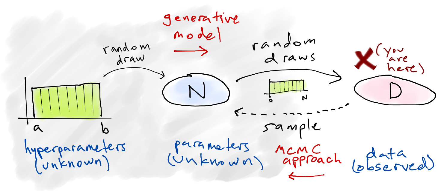
We start with a simplified story about how the data is generated — the generative model — and then attempt to infer specifics about that story (the parameters) based on what data we ended up with. In other words, we're constructing a simple model of how the universe could be arranged in such a way that we ended up seeing these four numbers, because we assume that random chance was involved and things could have turned out differently.

Here's our model:

Choose a number of tanks $N$ to exist in the world.
Of those $N$ , choose four that we happened to observe and call that data $D$ .

Of course, we actually start with the data $D$ rather than the parameter $N$ , and we could have observed these four serial numbers under many different choices of $N$ . The key is that some choices for $N$ are much more likely than others. For example, if $N$ was actually 5,000 then it would be a really odd coincidence that we happened to see all small numbers.

Solving it🔗

The Wikipedia article explains both the frequentist and Bayesian approaches, and the example in the Sampyl docs does a good job of explaining the setup for the Bayesian version. Here's the gist: we want to know the posterior probability of the number of tanks $N$ , given data $D$ on which tank serial numbers have been observed so far:

P (N ∣ D) \propto P (D ∣ N) P (N)

The right-hand side breaks down into two parts. The likelihood of observing all the serial numbers we saw is the product of the individual probabilities $D_{i}$ given the actual number of tanks in existence $N$ :

P (D ∣ N) = \prod_{i} P (D_{i} ∣ N)

P (D_{i} ∣ N) \sim DiscreteUniform (D, \min = 0, \max = N)

The prior over $N$ , which we know must be at least as high as the highest serial number we observed (call that $m$ ) but could be much higher:

$P (N) \sim DiscreteUniform (N, \min = m, \max = some big number)$

The MCMC strategy will be to try a bunch of different values for $N$ , see how likely they are (compared to one another), and assemble the results of the sampling into a distribution over $N$ . The solution implementation with Sampyl was interesting, but the project is still early so I wanted to give it a shot using two other popular MCMC libraries.

PyMC3🔗

PyMC seems to be most one of the most commonly used libraries for MCMC modeling in Python, and PyMC3 is the new version (still in beta). The tutorial in the project docs is a good read in and of itself, and Bayesian Methods for Hackers uses its predecessor PyMC2 extensively.

In [1]:

import numpy as np
import pymc3 as pm

# D: the data
y = np.array([10, 256, 202, 97])

model = pm.Model()
with model:
    
    # prior - P(N): N ~ uniform(max(y), 10000)
    # note: we use a large-ish number for the upper bound
    N = pm.DiscreteUniform("N", lower=y.max(), upper=10000)

    # likelihood - P(D|N): y ~ uniform(0, N)
    y_obs = pm.DiscreteUniform("y_obs", lower=0, upper=N, observed=y)

    # choose the sampling method - we have to use Metropolis-Hastings because
    # the variables are discrete
    step = pm.Metropolis()
    
    # we'll use four chains, and parallelize to four cores
    start = {"N": y.max()} # the highest number is a reasonable starting point
    trace = pm.sample(100000, step, start, chain=4, njobs=4)

 [-----------------100%-----------------] 100000 of 100000 complete in 20.4 sec

In [2]:

# summarize the trace
pm.summary(trace)

N:

  Mean             SD               MC Error         95% HPD interval
  -------------------------------------------------------------------
  
  384.280          186.753          1.928            [256.000, 688.000]

  Posterior quantiles:
  2.5            25             50             75             97.5
  |--------------|==============|==============|--------------|
  
  258.000        281.000        322.000        406.000        862.000

In [3]:

%matplotlib inline
from matplotlib import pyplot as plt

# plot the trace
burn_in = 10000  # throw away the first 10,000 samples
pm.traceplot(trace[burn_in:])
plt.show()

So the mean here was 384, and the median was 322.

PyStan🔗

PyStan "provides an interface to Stan, a package for Bayesian inference using the No-U-Turn sampler, a variant of Hamiltonian Monte Carlo." Stan, the underlying package, is designed to be a successor to JAGS, BUGS, and other hierarchical modeling tools.

Here's the same model implemented with PyStan. Two notes about how this differs:

The model specification is just a string written in the Stan sytax. PyStan is a thin wrapper that just handles sending off the model for compilation along with the data and then bringing back the results — it is not an attempt to write models in Python.
Stan doesn't currently have a convenient way to handle discrete parameters, which seems to be because the No-U-Turn Sampler (NUTS) and Hamiltonian Monte Carlo are designed for continuous variables only. For that reason, this formulation is for the continuous version of the problem and uses uniform instead of discrete uniform.

In [4]:

import pystan

ocode = """
data {
    int<lower=1> M;  // number of serial numbers observed
    real y[M];       // serial numbers
}
parameters {
    real<lower=max(y)> N;
}
model {
    N ~ uniform(max(y), 10000);  // P(N)
    y ~ uniform(0, N);           // P(D|N)
}
"""

data = {'y': y, 'M': len(y)}
fit = pystan.stan(model_code=ocode, data=data, init='init_r', iter=100000, warmup=1000, chains=4)
fit

Out[4]:

Inference for Stan model: anon_model_9faa1036eb89006b1e394cb29b5ab595.
4 chains, each with iter=100000; warmup=1000; thin=1; 
post-warmup draws per chain=99000, total post-warmup draws=396000.

       mean se_mean     sd   2.5%    25%    50%    75%  97.5%  n_eff   Rhat
N    383.94    0.33 207.36 258.37 282.63 323.44 406.62 869.66 396000    1.0
lp__ -19.45  1.3e-3   0.79 -21.71 -19.65 -19.15 -18.94 -18.89 396000    1.0

Samples were drawn using NUTS(diag_e) at Sat Dec 19 00:56:17 2015.
For each parameter, n_eff is a crude measure of effective sample size,
and Rhat is the potential scale reduction factor on split chains (at 
convergence, Rhat=1).

In [5]:

fig = fit.plot()
fig.set_size_inches((12, 2))

plt.tight_layout()
plt.show()

In [6]:

fit.extract()['N'].mean()

Out[6]:

383.94096084120298

The mean was again 384 and the median was 323, closely matching the results from above as expected.

Posts · Projects

Solving the Bayesian German Tank problem with PyMC and PyStan

19 Dec 2015

Problem set-up🔗

Solving it🔗

PyMC3🔗

PyStan🔗